
Getting Started with Structural Equation Modeling: Part 1
Introduction
For the analyst familiar with linear regression, fitting structural equation models can at first feel strange. In the R environment, fitting structural equation models involves learning new modeling syntax, new plotting syntax, and often a new data input method. However, after a quick reorientation, fitting structural equation models can be a powerful tool in the analyst’s toolkit.
This tutorial will cover getting set up and running a few basic models using lavaan in R.* Future tutorials will cover:
- constructing latent variables
- comparing alternate models
- multi-group analysis on larger datasets.
Setting up your enviRonment
Getting started using structural equation modeling (SEM) in R can be daunting. There are lots of different packages for implementing SEM in R and there are different features of SEM that a user might be interested in implementing. A few packages you might come across can be found on the CRAN Psychometrics Task View.
For those who want to just dive in the lavaan package seems to offer the most comprehensive feature set for most SEM users and has a well thought out and easy to learn syntax for describing SEM models. To install lavaan, we just run:
# Main version
install.packages("lavaan")

# Or to install the dev version
library(devtools)
install_github("lavaan", "yrosseel")
Read in the data
Once we load up the lavaan package, we need to read in the dataset. lavaan accepts two different types of data, either a standard R dataframe, or a variance-covariance matrix. Since the latter is unfamiliar to us coming from the standard lm linear modeling framework in R, we’ll start with reading in the simplest variance-covariance matrix possible and running a path analysis model.
library(lavaan)
mat1 <- matrix(c(1, 0, 0, 0.6, 1, 0, 0.33, 0.63, 1), 3, 3, byrow = TRUE)

colnames(mat1) <- rownames(mat1) <- c("ILL", "IMM", "DEP")

myN <- 500
print(mat1)
##      ILL  IMM DEP
## ILL 1.00 0.00   0
## IMM 0.60 1.00   0
## DEP 0.33 0.63   1
# Note that we only input the lower triangle of the matrix. This is
# sufficient though we could put the whole matrix in if we like
Now we have a variance-covariance matrix in our environment named mat1 and a variable myN corresponding to the number of observations in our dataset. Alternatively, we could provide R with the full dataset and it can derive mat1 and myN itself.
With this data we can construct two possible models:
- Depression (DEP) influences Immune System (IMM) influences Illness (ILL)
- IMM influences ILL influences DEP
Using SEM we can evaluate which model best explains the covariances we observe in our data above. Fitting models in lavaan is a two step process. First, we create a text string that serves as the lavaan model and follows the lavaan model syntax. Next, we give lavaan the instructions on how to fit this model to the data using either the cfa, lavaan, or sem functions. Here we will use the sem function. Other functions will be covered in a future post.
# Specify the model

mod1 <- "ILL ~ IMM \n        IMM ~ DEP"

# Give lavaan the command to fit the model
mod1fit <- sem(mod1, sample.cov = mat1, sample.nobs = 500)

# Specify model 2

mod2 <- "DEP ~ ILL\n        ILL ~ IMM"

mod2fit <- sem(mod2, sample.cov = mat1, sample.nobs = 500)
Now we have two objects stored in our environment for each model. We have the model string and the modelfit object. The model fit objects (mod1fit and mod2fit) are lavaan class objects. These are S4 objects with many supported methods, including the summary method which provides a lot of useful output:
# Summarize the model fit
summary(mod1fit)
## lavaan (0.5-14) converged normally after  12 iterations
##
##   Number of observations                           500
##
##   Estimator                                         ML
##   Minimum Function Test Statistic                2.994
##   Degrees of freedom                                 1
##   P-value (Chi-square)                           0.084
##
## Parameter estimates:
##
##   Information                                 Expected
##   Standard Errors                             Standard
##
##                    Estimate  Std.err  Z-value  P(>|z|)
## Regressions:
##   ILL ~
##     IMM               0.600    0.036   16.771    0.000
##   IMM ~
##     DEP               0.630    0.035   18.140    0.000
##
## Variances:
##     ILL               0.639    0.040
##     IMM               0.602    0.038
summary(mod2fit)
## lavaan (0.5-14) converged normally after  11 iterations
##
##   Number of observations                           500
##
##   Estimator                                         ML
##   Minimum Function Test Statistic              198.180
##   Degrees of freedom                                 1
##   P-value (Chi-square)                           0.000
##
## Parameter estimates:
##
##   Information                                 Expected
##   Standard Errors                             Standard
##
##                    Estimate  Std.err  Z-value  P(>|z|)
## Regressions:
##   DEP ~
##     ILL               0.330    0.042    7.817    0.000
##   ILL ~
##     IMM               0.600    0.036   16.771    0.000
##
## Variances:
##     DEP               0.889    0.056
##     ILL               0.639    0.040
One of the best ways to understand an SEM model is to inspect the model visually using a path diagram. Thanks to the semPlot package, this is easy to do in R.2 First, install semPlot:
# Official version
install.packages("semPlot")

# Or to install the dev version
library(devtools)
install_github("semPlot", "SachaEpskamp")
Next we load the library and make some path diagrams.
library(semPlot)
semPaths(mod1fit, what = "est", layout = "tree", title = TRUE, style = "LISREL")
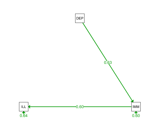
semPaths(mod2fit, what = "est", layout = "tree", title = TRUE, style = "LISREL")
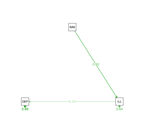
These two simple path models look great. But which is better? We can run a simple chi-square test on the lavaan objects mod1fit and mod2fit.
anova(mod1fit, mod2fit)
## Chi Square Difference Test
##
##         Df  AIC  BIC  Chisq Chisq diff Df diff Pr(>Chisq)
## mod1fit  1 3786 3803   2.99
## mod2fit  1 3981 3998 198.18        195       0     <2e-16 ***
## ---
## Signif. codes:  0 '***' 0.001 '**' 0.01 '*' 0.05 '.' 0.1 ' ' 1
We can see that very clearly we prefer Model 2. Let’s look at some properties of model 2 that we can access through the lavaan object with convenience functions.
# Goodness of fit measures
fitMeasures(mod2fit)
##              fmin             chisq                df            pvalue
##             0.198           198.180             1.000             0.000
##    baseline.chisq       baseline.df   baseline.pvalue               cfi
##           478.973             3.000             0.000             0.586
##               tli              nnfi               rfi               nfi
##            -0.243            -0.243             1.000             0.586
##              pnfi               ifi               rni              logl
##             0.195             0.587             0.586         -1986.510
## unrestricted.logl              npar               aic               bic
##         -1887.420             4.000          3981.020          3997.878
##            ntotal              bic2             rmsea    rmsea.ci.lower
##           500.000          3985.182             0.628             0.556
##    rmsea.ci.upper      rmsea.pvalue               rmr        rmr_nomean
##             0.703             0.000             0.176             0.176
##              srmr       srmr_nomean             cn_05             cn_01
##             0.176             0.176            10.692            17.740
##               gfi              agfi              pgfi               mfi
##             0.821            -0.075             0.137             0.821
##              ecvi
##             0.412
# Estimates of the model parameters
parameterEstimates(mod2fit, ci = TRUE, boot.ci.type = "norm")
##   lhs op rhs   est    se      z pvalue ci.lower ci.upper
## 1 DEP  ~ ILL 0.330 0.042  7.817      0    0.247    0.413
## 2 ILL  ~ IMM 0.600 0.036 16.771      0    0.530    0.670
## 3 DEP ~~ DEP 0.889 0.056 15.811      0    0.779    1.000
## 4 ILL ~~ ILL 0.639 0.040 15.811      0    0.560    0.718
## 5 IMM ~~ IMM 0.998 0.000     NA     NA    0.998    0.998
# Modification indices
modindices(mod2fit, standardized = TRUE)
##    lhs op rhs    mi    epc sepc.lv sepc.all sepc.nox
## 1  DEP ~~ DEP   0.0  0.000   0.000    0.000    0.000
## 2  DEP ~~ ILL 163.6 -0.719  -0.719   -0.720   -0.720
## 3  DEP ~~ IMM 163.6  0.674   0.674    0.675    0.674
## 4  ILL ~~ ILL   0.0  0.000   0.000    0.000    0.000
## 5  ILL ~~ IMM    NA     NA      NA       NA       NA
## 6  IMM ~~ IMM   0.0  0.000   0.000    0.000    0.000
## 7  DEP  ~ ILL   0.0  0.000   0.000    0.000    0.000
## 8  DEP  ~ IMM 163.6  0.675   0.675    0.675    0.676
## 9  ILL  ~ DEP 163.6 -0.808  -0.808   -0.808   -0.808
## 10 ILL  ~ IMM   0.0  0.000   0.000    0.000    0.000
## 11 IMM  ~ DEP 143.8  0.666   0.666    0.666    0.666
## 12 IMM  ~ ILL   0.0  0.000   0.000    0.000    0.000
That’s it. From inputing a variance-covariance matrix to fitting a model, drawing a path diagram, comparing to alternate models, and finally inspecting the parameters of the preferred model. lavaan is an amazing project which adds great capabilities to R. These will be explored in future posts.
Appendix
citation(package = "lavaan")
##
## To cite lavaan in publications use:
##
##   Yves Rosseel (2012). lavaan: An R Package for Structural
##   Equation Modeling. Journal of Statistical Software, 48(2), 1-36.
##   URL http://www.jstatsoft.org/v48/i02/.
##
## A BibTeX entry for LaTeX users is
##
##   @Article{,
##     title = {{lavaan}: An {R} Package for Structural Equation Modeling},
##     author = {Yves Rosseel},
##     journal = {Journal of Statistical Software},
##     year = {2012},
##     volume = {48},
##     number = {2},
##     pages = {1--36},
##     url = {http://www.jstatsoft.org/v48/i02/},
##   }
citation(package = "semPlot")
##
## To cite package 'semPlot' in publications use:
##
##   Sacha Epskamp (2013). semPlot: Path diagrams and visual analysis
##   of various SEM packages' output. R package version 0.3.3.
##   https://github.com/SachaEpskamp/semPlot
##
## A BibTeX entry for LaTeX users is
##
##   @Manual{,
##     title = {semPlot: Path diagrams and visual analysis of various SEM packages' output},
##     author = {Sacha Epskamp},
##     year = {2013},
##     note = {R package version 0.3.3},
##     url = {https://github.com/SachaEpskamp/semPlot},
##   }
##
## ATTENTION: This citation information has been auto-generated from
## the package DESCRIPTION file and may need manual editing, see
## 'help("citation")'.
sessionInfo()
## R version 3.0.1 (2013-05-16)
## Platform: x86_64-w64-mingw32/x64 (64-bit)
##
## locale:
## [1] LC_COLLATE=English_United States.1252
## [2] LC_CTYPE=English_United States.1252
## [3] LC_MONETARY=English_United States.1252
## [4] LC_NUMERIC=C
## [5] LC_TIME=English_United States.1252
##
## attached base packages:
## [1] stats     graphics  grDevices utils     datasets  methods   base
##
## other attached packages:
## [1] semPlot_0.3.3  lavaan_0.5-14  quadprog_1.5-5 pbivnorm_0.5-1
## [5] mnormt_1.4-5   boot_1.3-9     MASS_7.3-28    knitr_1.4.1
##
## loaded via a namespace (and not attached):
##  [1] car_2.0-18       cluster_1.14.4   colorspace_1.2-2 corpcor_1.6.6
##  [5] digest_0.6.3     ellipse_0.3-8    evaluate_0.4.7   formatR_0.9
##  [9] grid_3.0.1       Hmisc_3.12-2     igraph_0.6.5-2   jpeg_0.1-6
## [13] lattice_0.20-23  lisrelToR_0.1.4  plyr_1.8         png_0.1-6
## [17] psych_1.3.2      qgraph_1.2.3     rockchalk_1.8.0  rpart_4.1-2
## [21] sem_3.1-3        stats4_3.0.1     stringr_0.6.2    tools_3.0.1
## [25] XML_3.98-1.1
- *https://lavaan.ugent.be/